![]()
The noaaoceans package is designed to facilitate access to various National Oceanic and Atmospheric Administration (NOAA) data sources. The current version focuses on accessing data from the CO-OPS API. The package also facilitates the collection of basic metadata for each of the stations that collect the data available in the API.
The current release of noaaoceans can be installed from CRAN.
install.packages('noaaoceans')The development version can be installed via GitHub with remotes
remotes::install_github('warlicks/noaaoceans')library(noaaoceans)
library(dplyr)
library(ggplot2)
library(maps)
library(mapdata)
# Get a list of all the stations.
station_df <- list_coops_stations()
# Filter to stations in Washington with Water Temp Sensor
wa_station <- station_df %>%
filter(station_state == 'WA' & water_temp == '1')
wa_station %>% dplyr::as_tibble(.) %>% head()
#> # A tibble: 6 x 15
#> station_id station_names station_state station_lat station_long
#> <chr> <chr> <chr> <chr> <chr>
#> 1 9440422 Longview WA 46.1061 -122.9542
#> 2 9440910 Toke Point WA 46.7075 -123.9669
#> 3 9441102 Westport WA 46.9043 -124.1051
#> 4 9442396 La Push, Qui… WA 47.913 -124.6369
#> 5 9443090 Neah Bay WA 48.3703 -124.6019
#> 6 9444090 Port Angeles WA 48.125 -123.44
#> # … with 10 more variables: date_established <chr>, water_level <chr>,
#> # winds <chr>, air_temp <chr>, water_temp <chr>, air_pressure <chr>,
#> # conductivity <chr>, visibility <chr>, humidity <chr>, air_gap <chr># Create an empty storage data frame.
water_temp <- data.frame()
# Loop through the station and call the API for each station
for (i in wa_station$station_id) {
query_df <- query_coops_data(station_id = i,
start_date = '20181201',
end_date = '20181231',
data_product = 'water_temperature',
interval = 'h') # hourly readings
# Add current station results to the storage data frame
water_temp <- water_temp %>% bind_rows(., query_df)
}
water_temp %>% as_tibble(.) %>% head()
#> # A tibble: 6 x 4
#> t v f station
#> <chr> <chr> <chr> <chr>
#> 1 2018-12-01 00:00 48.4 0,0,0 9440422
#> 2 2018-12-01 01:00 48.4 0,0,0 9440422
#> 3 2018-12-01 02:00 48.4 0,0,0 9440422
#> 4 2018-12-01 03:00 48.4 0,0,0 9440422
#> 5 2018-12-01 04:00 48.4 0,0,0 9440422
#> 6 2018-12-01 05:00 48.4 0,0,0 9440422# Correct data types.
water_temp <- water_temp %>%
mutate(v = as.numeric(v), t = as.POSIXct(t))
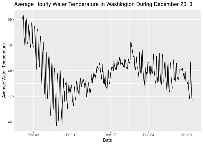
water_temp %>%
group_by(t) %>%
# Compute the hourly average.
summarise(avg_temp = mean(v, na.rm = TRUE)) %>%
# Plot the hourly average.
ggplot(aes(x = t, y = avg_temp)) +
geom_path() +
labs(x = "Date",
y = 'Average Water Temperature',
title = 'Average Hourly Water Temperature In Washington During December 2018')
#> `summarise()` ungrouping output (override with `.groups` argument)