
![]()
![]()
![]()
The Concise Spatial QUery And REpresentation System (c-squares) are identifiers that correspond with cells in a global grid. The system was developed by CSIRO Oceans & Atmosphere and divides the globe in rectangles of 10 by 10 degrees (longitude and latitude in WGS84). It is a hierarchical system, meaning that higher resolutions are also supported, as long as its cell size is a tenfold of 1 or 5 degrees (i.e., cells can have the following sizes in degrees: 10, 5, 1, 0.5, 0.1, etc.).
The c-squares format is a well defined exchange format for spatial raster data, it allows for light-weight text querying / aggregation and expansion to different resolutions. The csquare R package facilitates the translation of c-square code into spatial information (sf and stars) and vice versa.
For more technical information on c-squares, please consult the Wikipedia page or the CSIRO c-squares page.
Get CRAN version
install.packages("csquares")Get development version from r-universe
install.packages("csquares", repos = c("https://pepijn-devries.r-universe.dev", "https://cloud.r-project.org"))The example below is based on killer whale realm data extracted from the publication by Costello et al. (2017).
The orca data set itself is not provided as a
simple features object,
which is commonly used in R for spatial analyses. Instead, spatial
information is encoded in the c-squares format. The example below shows
how these codes can be decoded in a spatially explicit format which can
be used for subsequent analyses.
library(csquares)
library(sf)
library(ggplot2)

## Convert the data.frame into a csquares object
orca_csq <- as_csquares(orca, csquares = "csquares")

## Convert the csquares object into a simple features object
## and transform to Robinson's projection
orca_sf <-
  orca_csq |>
  st_as_sf() |>
  st_transform(crs = "+proj=robin +lon_0=0 +x_0=0 +y_0=0")

## Make a plot of the spatial data
ggplot(orca_sf) +
  geom_sf(aes(fill = orcinus_orca)) +
  coord_sf(expand = FALSE)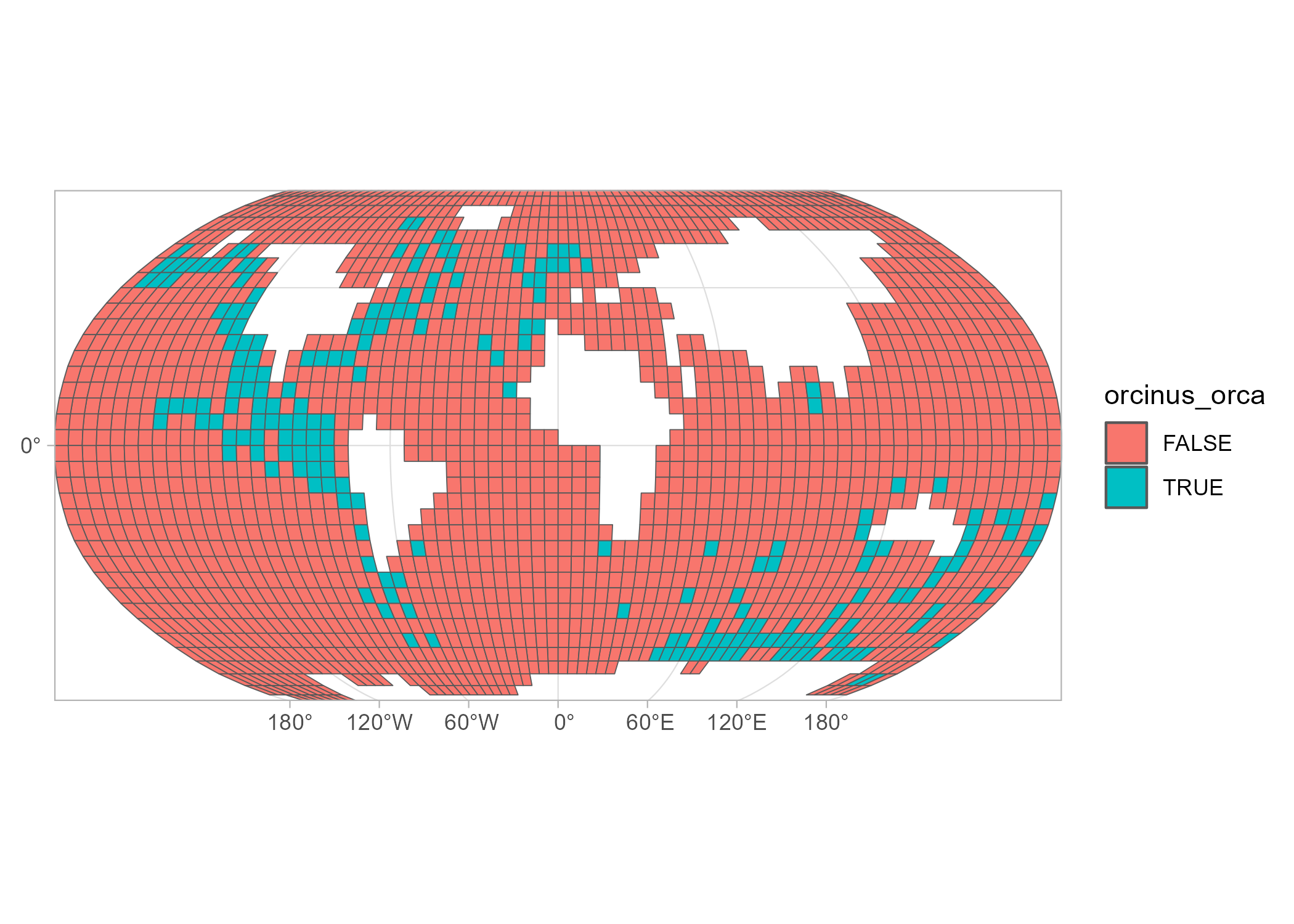
The example above uses existing data with specified c-square codes. You can also create a raster with c-square codes from scratch. The example below shows how to create a 0.1 x 0.1 degrees raster for a specific bounding box.
st_bbox(c(xmin = 5.0, xmax = 5.5, ymin = 52.5, ymax = 53), crs = 4326) |>
  new_csquares(resolution = 0.1)
#> stars object with 2 dimensions and 1 attribute
#> attribute(s):
#>   csquares
#>  Length:25
#>  Class :character
#>  Mode  :character
#> dimension(s):
#>   from to offset delta refsys x/y
#> x    1  5      5   0.1 WGS 84 [x]
#> y    1  5     53  -0.1 WGS 84 [y]