
boiwsa is an R package for seasonal adjustment and
forecasting of weekly data. It provides a simple, easy-to-use interface
for calculating the seasonally adjusted estimates, as well as a number
of diagnostic tools for evaluating the quality of the adjustments. In
this tutorial we illustrate its functionality in seasonal adjustment and
forecasting of the weekly data.
The seasonal adjustment procedure approach aligns closely with the locally-weighted least squares procedure introduced by Cleveland et al. (2014) albeit with several adjustments. Firstly, instead of relying on differencing to detrend the data, we opt for a more explicit approach by directly estimating the trend through smoothing techniques. Secondly, we incorporate a variation of Discount weighted regression (Harrison and Johnston, 1984) to enable the seasonal component to evolve dynamically over time.
We consider the following decomposition model of the observed series \(y_{t}\):
\[ y_{t}=T_{t}+S_{t}+H_{t}+O_{t}+I_{t}, \]
where \(T_{t}\), \(S_{t}\), \(H_{t}\), \(O_{t}\) and \(I_{t}\) represent the trend, seasonal, outlier, holiday- and trading-day, and irregular components, respectively. To evade ambiguity, it is important to note that in weekly data, \(t\) typically denotes the date of the last day within a given week. The seasonal component is specified using trigonometric variables as:
\begin{eqnarray*}
S_{t} &=&\sum_{k=1}^{K}\left( \alpha _{k}^{y}\sin (\frac{2\pi kD_{t}^{y}}{
n_{t}^{y}})+\beta _{k}^{y}\cos (\frac{2\pi kD_{t}^{y}}{n_{t}^{y}})\right) +
\\
&&\sum_{l=1}^{L}\left( \alpha _{l}^{m}\sin (\frac{2\pi lD_{t}^{m}}{n_{t}^{m}}
)+\beta _{l}^{m}\cos (\frac{2\pi lD_{t}^{m}}{n_{t}^{m}})\right) ,
\end{eqnarray*}
where \(D_{t}^{y}\) and \(D_{t}^{m}\) are the day of the year and the day of the month, and \(n_{t}^{y}\) and \(n_{t}^{m}\) are the number of days in the given year or month. Thus, the seasonal adjustment procedure takes into account the existence of two cycles, namely intrayearly and intramonthly.
Like the X-11 method (Ladiray and Quenneville, 2001), the
boiwsa procedure uses an iterative principle to estimate
the various components. The seasonal adjustment algorithm comprises
eight steps, which are documented below:
Step 1: Estimation of trend (\(T_{t}^{(1)}\)) using
stats::supsmu().
Step 2: Estimation of the Seasonal-Irregular component:
\[y_{t}-T_{t}^{(1)}=S_{t}+H_{t}+O_{t}+I_{t}\]
Step 2*: Searching for additive outliers using the method proposed by Findley et al. (1998)
Step 2**: Identifying the optimal number of trigonometric variables
Step 3: Calculation of seasonal factors, along with other potential factors such as \(H_{t}\) or \(O_{t}\), is done through DWR on the seasonal-irregular component extracted in Step 2. In this application, the discounting rate decays over the years. For each year \(t\) and the observed year \(\tau\), a geometrically decaying weight function is represented as: \(w_{t}=r^{|t-\tau|}\), where \(r \in (0,1]\). Several important points are worth mentioning. First, when \(r=1\), the method simplifies to ordinary least squares regression with constant seasonality. On the contrary, smaller values of \(r\) permit a more rapid rate of change in the seasonal component. However, it is advised against setting it below 0.5 to prevent overfitting. In addition, the choice of \(r\) affects the strength of revisions in the seasonally adjusted data, with higher values of \(r\) leading to potentially stronger revisions. Second, our methodology differs from the conventional one-way discounting, enabling the inclusion of future observations in the computation of seasonal factors. This approach circumvents the limitations of the forecasting methods discussed in Bandara et al. (2024). Finally, the choice of year-based discounting is driven by the fact that in traditional discount-weighted regression, even with a conservative choice of \(r=0.95\), in weekly data, observations separated by more than 2 years would carry nearly negligible weight. Therefore, the use of year-based discounting prevents an overly rapid decay which may potentially lead to unstable estimates of the seasonal component.
Step 4: Estimation of trend (\(T_{t}^{(2)}\)) from seasonally and outlier
adjusted series using stats::supsmu() function (R Core
Team,
Step 5: Estimation of the Seasonal-Irregular component: \[y_{t}-T_{t}^{(2)}=S_{t}+H_{t}+O_{t}+I_{t}\]
Step 6: Computing the final seasonal factors (and possibly other factors such as \(H_{t}\) or \(O_{t}\)) using discount weighted regression, as in step 3.
Step 7: Estimation of the final seasonally adjusted series: \[y_{t}-S_{t}-H_{t}\]
Step 8: Computing final trend (\(T_{t}^{(3)}\)) estimate from seasonally and
outlier adjusted series using stats::supsmu().
To install boiwsa, you can use devtools:
# install.packages("devtools")
devtools::install_github("timginker/boiwsa")
Alternatively, you can clone the repository and install the package from source:
git clone https://github.com/timginker/boiwsa.git
cd boiwsa
R CMD INSTALL .Using boiwsa is simple. First, load the
boiwsa package:
library(boiwsa)Next, load your time series data into a data frame object. Here is an
example that is based on the gasoline data from the US
Energy Information Administration that we copied from the from the
fpp2 package:
data("gasoline.data")
plot(gasoline.data$date,
     gasoline.data$y,
     type="l"
     ,xlab="Year",
     ylab=" ",
     main="Weekly US gasoline production")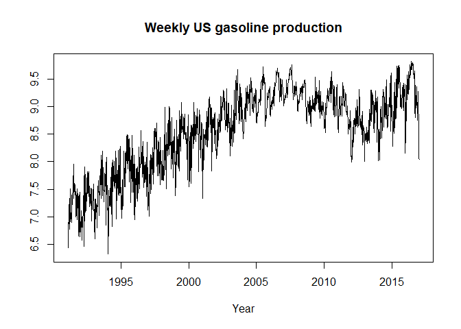
Once you have your data loaded, you can use the boiwsa
function to perform weekly seasonal adjustment:
res <- boiwsa(
  x = gasoline.data$y,
  dates = gasoline.data$date
)
In general, the procedure can be applied with minimum interventions
and requires only the series to be adjusted (x argument)
and the associated dates (dates argument) provided in a
date format. Unless specified otherwise (i.e.,
my.k_l = NULL), the procedure automatically identifies the
best number of trigonometric variables to model the intra-yearly (\(K\)) and intra-monthly (\(L\)) seasonal cycles based on the Akaike
Information Criterion corrected for small sample sizes (AICc). The
information criterion can be adjusted through the ic
option. Like other software, there are three options: “aic”, “aicc”, and
“bic”. The weighting decay rate is specified by r. By
default \(r=0.8\) which is similar to
what is customary in the literature (see Ch. 2 in Harvey (1990)).
In addition, the procedure automatically searches for additive
outliers (AO) using the method described in Appendix C of Findley et
al. (1998). To disable the automatic AO search, set
auto.ao.search = F. To add user-defined AOs, use the
ao.list option. As suggested by Findley et al. (1998), the
\(t\)-statistic threshold for outlier
search is by default set to \(3.8\).
However, since high-frequency data are generally more noisy (Proietti
and Pedregal, 2023), it could be advantageous to consider setting a
higher threshold by adjusting the out.threshold
argument.
The boiwsa function returns an S3 class object
containing the results. The seasonally adjusted series is stored in a
vector called sa. The estimated seasonal factors are stored
as sf. In addition, the user can see the number of
trigonometric terms chosen in automatic search (my.k_l) and
the position of additive outliers (ao.list) found by the
automatic routine.
After the seasonal adjustment, we can plot the adjusted data to visualize the seasonal pattern:
plot(res)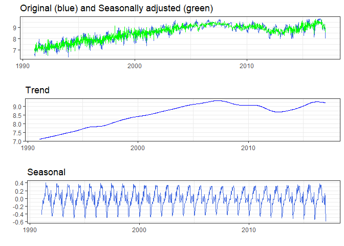
To assess the quality of the adjustment, we can plot the autoregressive spectrum of the original and seasonally adjusted data, as illustrated in the code below:
plot_spec(res)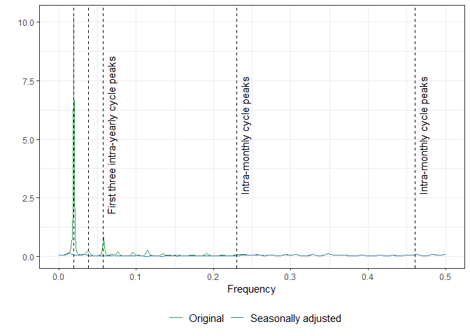
It is evident that the series originally had a single intra-yearly seasonal cycle, but this component was completely removed by the procedure.
We can also inspect the output to check if the number of trigonometric terms chosen by the automatic procedure matches our visual findings:
print(res)
#>
#>  number of yearly cycle variables:  12
#>  number of monthly cycle variables:  0
#>  list of additive outliers:  1998-03-28
As can be seen, the number of yearly terms, \(K\), is 12 and the number of monthly terms is zero, which is consistent with the observed spectrum.
Here, we consider the weekly number of initial registrations at the Israeli Employment Service. Registration and reporting at the Employment Service are mandatory prerequisites for individuals seeking to receive an unemployment benefit. Therefore, applicants are expected to register promptly after their employment has been terminated. Given that most employment contracts conclude toward the end of the month, an increased number of applications is anticipated at the beginning of the month, leading to an intra-monthly seasonal pattern. Additionally, as can be seen in the Figure below, on an annual basis, three distinct peaks are observed, with the final one occurring in August. This peak is closely tied to seasonal workers, leading to the creation of an intra-yearly cycle.
library(tidyverse)
#> ── Attaching core tidyverse packages ──────────────────────── tidyverse 2.0.0 ──
#> ✔ dplyr     1.1.4     ✔ readr     2.1.4
#> ✔ forcats   1.0.0     ✔ stringr   1.5.1
#> ✔ ggplot2   3.4.4     ✔ tibble    3.2.1
#> ✔ lubridate 1.9.3     ✔ tidyr     1.3.0
#> ✔ purrr     1.0.2
#> ── Conflicts ────────────────────────────────────────── tidyverse_conflicts() ──
#> ✖ dplyr::filter() masks stats::filter()
#> ✖ dplyr::lag()    masks stats::lag()
#> ℹ Use the conflicted package (<http://conflicted.r-lib.org/>) to force all conflicts to become errors
ggplot() +
  geom_line(aes(
    x = lbm$date,
    y = lbm$IES_IN_W_ADJ
  ), color = "royalblue") +
  theme_bw() +
  ylab("Number of claims per week") +
  xlab("Year")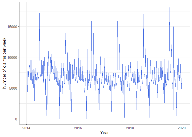
Furthermore, each year, there are two weeks in which the activity
plunges to nearly zero due to the existence of two moving holidays
associated with Rosh Hashanah and Pesach. Moreover, a working day effect
is expected, which leads to a reduced number of applications in weeks
with fewer working days. These effects are captured and modeled through
additional variables generated by the dedicated functions in
boiwsa.
To generate a working day variable, we use the
boiwsa::simple_td function, designed to aggregate the count
of full working days within a week and normalize it. This function
requires two parameters: the data dates and a data.frame
object containing information about working days. The
data.frame should be in a daily frequency and contain two
columns: “date” and “WORKING_DAY_PART”. For a complete working day, the
“WORKING_DAY_PART” column should be assigned a value of 1, for a half
working day 0.5, and for a holiday, the value should be set to 0.
Moving holiday variables can be created using the
boiwsa::genhol function. These variables are computed using
the Easter formula in Table 2 of Findley et al. (1998), with the
calendar centering to avoid bias, as indicated in the documentation. In
the present example, the impact of each holiday is concentrated within a
single week, resulting in a noticeable drop and subsequent increase in
the number of registrations during the following week. To account for
this effect, we employ dummy variables that are globally centered. These
dummy variables are created using a custom function -
boiwsa::my_rosh, which is created for this illustrative
scenario.
The code below illustrates the entire process based on the
boiwsa::lbm dataset: creation of working day adjustment
variables using the boiwsa::simple_td function; creation of
moving holiday variables using the dedicated functions, and adding the
combined input into the boiwsa::boiwsa function.
# creating an input for simple_td
dates_il %>%
  select(DATE_VALUE, ISR_WORKING_DAY_PART) %>%
  `colnames<-`(c("date", "WORKING_DAY_PART")) %>%
  mutate(date = as.Date(date)) -> df.td
# creating a matrix with a working day variable
td <- simple_td(dates = lbm$date, df.td = df.td)

# generating the Rosh Hashanah and Pesach moving holiday variables
rosh <- my_rosh(
  dates = lbm$date,
  holiday.dates = holiday_dates_il$rosh
)
# renaming (make sure that all the variables in H have distinct names)
colnames(rosh) <- paste0("rosh", colnames(rosh))

pesach <- my_rosh(
  dates = lbm$date,
  holiday.dates = holiday_dates_il$pesah,
  start = 3, end = -1
)
colnames(pesach) <- paste0("pesach", colnames(pesach))


# combining the prior adjustment variables in a single matrix
H <- as.matrix(cbind(rosh[, -1], pesach[, -1], td[, -1]))
# running seasonal adjustment routine
res <- boiwsa(
  x = lbm$IES_IN_W_ADJ,
  dates = lbm$date,
  H = H,
  out.threshold = 5
)
Subsequently, we can visually examine the results of the procedure:
plot(res)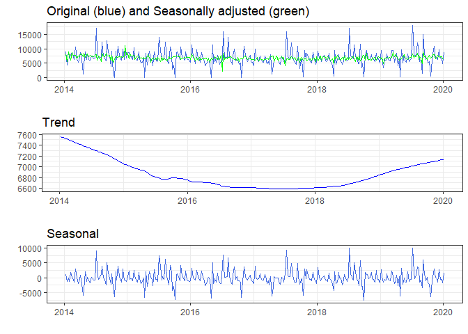
As we can see in the plot, the procedure has successfully eliminated the annual and monthly seasonal cycles, along with the influences of moving holidays.
Following a thorough visual examination of the seasonally adjusted data, we can now move forward with the spectrum diagnostics. As illustrated in the Figure below, corroborating our initial analysis of potential underlying seasonal patterns, it becomes evident that the data has two distinct seasonal cycles. Additionally, it is noteworthy that our procedure successfully removed the corresponding peaks, thereby highlighting its effectiveness.
plot_spec(res)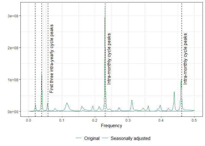
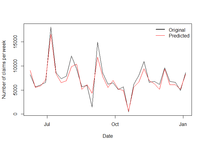
It is also possible to forecast weekly data using the predict method
for boiwsa. The prediction is based on the
forecast::auto.arima model fitted to the seasonally and
outlier-adjusted data, which is then combined with the seasonal factor
estimates from boiwsa.
The code below illustrates the entire process:
x <- boiwsa::lbm$IES_IN_W_ADJ
dates <- boiwsa::lbm$date
# train-test split (using 90% of observations for train)
n_train <- round(length(x) * 0.9)
n_test <- (length(x) - n_train)
h_train <- H[1:n_train, ]
h_test <- tail(H, n_test)
x_train <- x[1:n_train]
x_test <- tail(x, n_test)
dates_train <- dates[1:n_train]
dates_test <- tail(dates, n_test)

fit <- boiwsa(
  x = x_train,
  dates = dates_train,
  H = h_train
)

fct <- predict(fit,
  n.ahead = n_test,
  new_H = h_test
)

# Visualizing predictions

plot(dates_test,
     x_test,type="l",
     ylab="Number of claims per week",
     xlab="Date")
lines(dates_test,
      fct$forecast$mean,
      col="red")
legend(
  "topright",
  legend = c("Original", "Predicted"),
  lwd = c(2, 1),
  col = c("black", "red"),
  bty = "n"
)
Bandara, K., Hyndman, R. J. and C. Bergmeir (2024). MSTL: A seasonal-trend decomposition algorithm for time series with multiple seasonal patterns. International Journal of Operational Research, 2024. In press.
Cleveland, W.P., Evans, T.D. and S. Scott (2014). Weekly Seasonal Adjustment-A Locally-weighted Regression Approach (No. 473). Bureau of Labor Statistics.
Findley, D.F., Monsell, B.C., Bell, W.R., Otto, M.C. and B.C Chen (1998). New capabilities and methods of the X-12-ARIMA seasonal-adjustment program. Journal of Business & Economic Statistics, 16(2), pp.127-152.
Harrison, P. J. and F. R. Johnston (1984). Discount weighted regression. Journal of the Operational Research Society 35(10), 923–932.
Hyndman, R. (2023). fpp2: Data for “Forecasting: Principles and Practice” (2nd Edition). R package version 2.5.
Harvey, A. C. (1990). Forecasting, structural time series models and the Kalman filter. Cambridge University Press.
Ladiray, D. and B. Quenneville (2001). Seasonal adjustment with the X-11 method.
Proietti, T. and D. J. Pedregal (2023). Seasonality in High Frequency Time Series. Econometrics and Statistics, 27: 62–82, 2023.
R Core Team (2013). R: A Language and Environment for Statistical Computing. Vienna, Austria: R Foundation for Statistical Computing. ISBN 3-900051-07-0.
The views expressed here are solely of the author and do not necessarily represent the views of the Bank of Israel.
Please note that boiwsa is still under development and
may contain bugs or other issues that have not yet been resolved. While
we have made every effort to ensure that the package is functional and
reliable, we cannot guarantee its performance in all situations.
We strongly advise that you regularly check for updates and install any new versions that become available, as these may contain important bug fixes and other improvements. By using this package, you acknowledge and accept that it is provided on an “as is” basis, and that we make no warranties or representations regarding its suitability for your specific needs or purposes.