FLASH-MM is a method (package name: FLASHMM) for analysis of single-cell differential expression using a linear mixed-effects model (LMM). The mixed-effects model is a powerful tool in single-cell studies due to their ability to model intra-subject correlation and inter-subject variability.
FLASHMM package provides two functions, lmm and lmmfit, for fitting LMM. The lmm function uses summary statistics as arguments. The lmmfit function is a wrapper function of lmm, which directly uses cell-level data and computes the summary statistics inside the function. The lmmfit function is simple to be operated but it has a limitation of memory use. For extremely large scale data, it is recommended to precompute and store the summary statistics and then use lmm function to fit LMM.
In summary, FLASHMM package provides the following main functions.
You can install FLASHMM package from CRAN:
install.packages("FLASHMM")Or the development version from GitHub:
devtools::install_github("https://github.com/Baderlab/FLASHMM")This is a basic example which shows you how to use FLASHMM to perform single-cell differential expression analysis.
library(FLASHMM)Simulate a multi-sample multi-cell-cluster scRNA-seq dataset that contains 25 samples and 4 clusters (cell-types) with 2 treatments.
set.seed(2412)
dat <- simuRNAseq(nGenes = 50, nCells = 1000, nsam = 25, ncls = 4, ntrt = 2, nDEgenes = 6)
#> Message: the condition B is treated.
names(dat)
#> [1] "ref.mean.dispersion" "metadata"            "counts"
#> [4] "DEgenes"             "treatment"

#counts and meta data
counts <- dat$counts
metadata <- dat$metadata
head(metadata)
#>       sam cls trt libsize
#> Cell1  B1   4   B     117
#> Cell2  A6   3   A      75
#> Cell3  A2   1   A     101
#> Cell4  B8   1   B      80
#> Cell5 B11   4   B     123
#> Cell6  A4   3   A     113
rm(dat)
The simulated data contains
The analyses involve following steps: LMM design, LMM fitting, and hypothesis testing.
1. Model design
Y <- log(counts + 1)
X <- model.matrix(~ 0 + log(libsize) + cls + cls:trt, data = metadata)
Z <- model.matrix(~ 0 + sam, data = metadata)
d <- ncol(Z)
2. LMM fitting
Option 1: Fit LMMs with lmmfit function using cell-level data.
fit <- lmmfit(Y, X, Z, d = d)Option 2: Fit LMMs with lmm function using summary-level data.
##(1) Computing summary statistics
n <- nrow(X)
XX <- t(X)%*%X; XY <- t(Y%*%X)
ZX <- t(Z)%*%X; ZY <- t(Y%*%Z); ZZ <- t(Z)%*%Z
Ynorm <- rowSums(Y*Y)

##(2) Fitting LMMs
fitss <- lmm(XX, XY, ZX, ZY, ZZ, Ynorm = Ynorm, n = n, d = d)

identical(fit, fitss)
#> [1] TRUE
3. Hypothesis testing
## Testing coefficients (fixed effects)
test <- lmmtest(fit)
# head(test)

## The t-value and p-values are identical with those provided in the LMM fit.
range(test - cbind(t(fit$coef), t(fit$t), t(fit$p)))
#> [1] 0 0

fit$p[, 1:4]
#>                     Gene1        Gene2        Gene3        Gene4
#> log(libsize) 0.0003936946 1.226867e-09 0.0003216502 4.036515e-05
#> cls1         0.0158766072 1.300111e-06 0.0209667982 7.686618e-03
#> cls2         0.0095791682 7.060831e-07 0.0248727531 1.220264e-02
#> cls3         0.0106867912 5.971329e-07 0.0319158551 9.862323e-03
#> cls4         0.0145925607 6.556356e-07 0.0266262016 7.087769e-03
#> cls1:trtB    0.3846324624 7.144869e-01 0.8795840262 3.319065e-01
#> cls2:trtB    0.0387066712 2.726210e-01 0.9114719020 4.580478e-01
#> cls3:trtB    0.1322220329 1.338870e-01 0.7144983040 3.745743e-01
#> cls4:trtB    0.7442524470 9.307711e-02 0.6485383571 5.182577e-01

# fit$coef[, 1:4] fit$t[, 1:4]
Using contrasts: We can make comparisons using contrasts. For example, the effects of treatment B vs A in all clusters can be tested using the contrast constructed as follows.
ct <- numeric(ncol(X))
index <- grep("B", colnames(X))
ct[index] <- 1/length(index)

test <- lmmtest(fit, contrast = ct)
head(test)
#>             _coef         _t        _p
#> Gene1  0.09445436  1.4753256 0.1404426
#> Gene2  0.10333114  1.4540794 0.1462409
#> Gene3 -0.02117872 -0.2900354 0.7718498
#> Gene4  0.10281315  0.9531558 0.3407436
#> Gene5 -0.12106061 -1.3918602 0.1642770
#> Gene6 0.06756558 1.1553425 0.2482287To use the maximum likelihood (ML) method to fit the LMM, set method = ‘ML’ in the lmm and lmmfit functions.
##Fitting LMM using ML method
fit1 <- lmmfit(Y, X, Z, d = d, method = "ML")If appropriate, for example, we also take account of the measurement time as a random effect within a subject, we may fit data using the LMM with two-component random effects.
## Design matrix for two-component random effects: Suppose the data contains
## the measurement time points, denoted as 'time', which are randomly
## generated.

set.seed(2508)
n <- nrow(metadata)
metadata$time <- sample(1:2, n, replace = TRUE)
Z <- model.matrix(~0 + sam + sam:time, data = metadata)
d <- c(ncol(Z)/2, ncol(Z)/2)  #dimension

## Fit the LMM with Two-component random effects.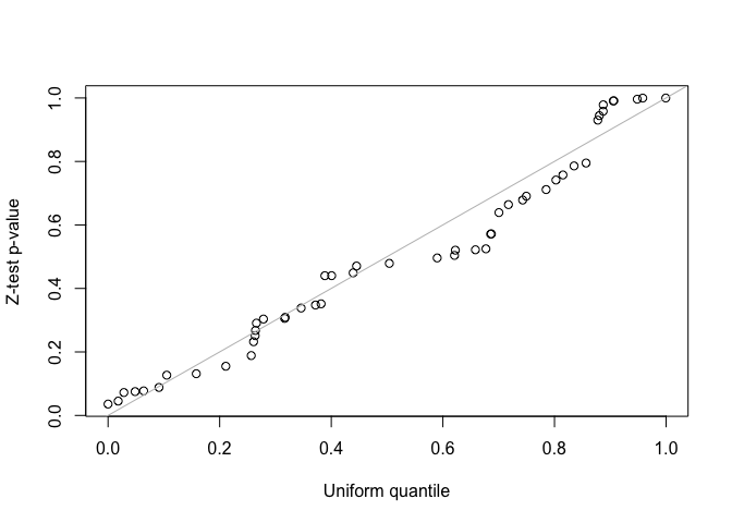
fit2 <- lmmfit(Y, X, Z, d = d, method = "ML")We use both z-test and likelihood ratio test (LRT) to test the second variance component in the LMM with two-component random effects. Since the simulated data was generated by the LMM with single-component random effects, the second variance component should be zero. For the LRT test, the two nested models must be fitted using the same method, either REML or ML, and use the same design matrix, \(X\), when using REML method.
##(1) z-test for testing the second variance component
##Z-statistics for the second variance component
i <- grep("var2", rownames(fit2$theta))
z <- fit2$theta[i, ]/fit2$se.theta[i, ]
##One-sided z-test p-values for hypotheses:
##H0: theta <= 0 vs H1: theta > 0
p <- pnorm(z, lower.tail = FALSE)

##(2) LRT for testing the second variance component
LRT <- 2*(fit2$logLik - fit1$logLik)
pLRT <- pchisq(LRT, df = 1, lower.tail = FALSE)

##QQ-plot
qqplot(runif(length(p)), p, xlab = "Uniform quantile", ylab = "Z-test p-value")
abline(0, 1, col = "gray")
qqplot(runif(length(pLRT)), pLRT, xlab = "Uniform quantile", ylab = "LRT p-value")
abline(0, 1, col = "gray")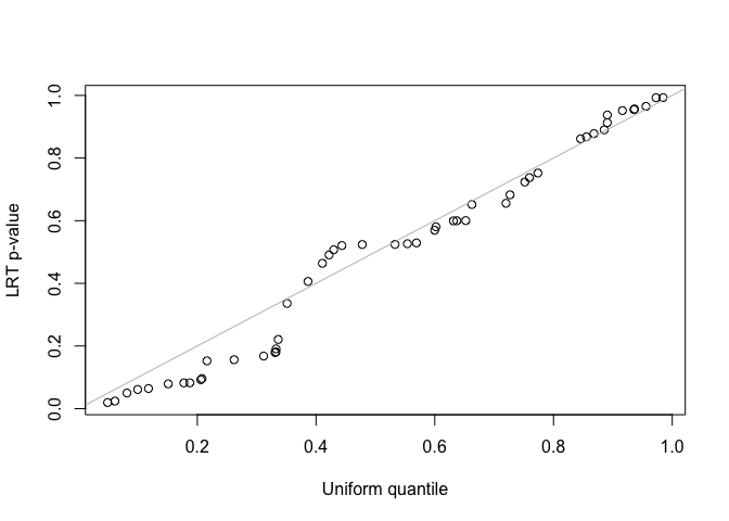
sessionInfo()
#> R version 4.4.3 (2025-02-28)
#> Platform: x86_64-apple-darwin20
#> Running under: macOS Monterey 12.7.6
#>
#> Matrix products: default
#> BLAS:   /Library/Frameworks/R.framework/Versions/4.4-x86_64/Resources/lib/libRblas.0.dylib
#> LAPACK: /Library/Frameworks/R.framework/Versions/4.4-x86_64/Resources/lib/libRlapack.dylib;  LAPACK version 3.12.0
#>
#> locale:
#> [1] en_US.UTF-8/en_US.UTF-8/en_US.UTF-8/C/en_US.UTF-8/en_US.UTF-8
#>
#> time zone: America/Toronto
#> tzcode source: internal
#>
#> attached base packages:
#> [1] stats     graphics  grDevices utils     datasets  methods   base
#>
#> other attached packages:
#> [1] FLASHMM_1.2.1
#>
#> loaded via a namespace (and not attached):
#>  [1] Matrix_1.7-3       miniUI_0.1.2       compiler_4.4.3     promises_1.3.3
#>  [5] Rcpp_1.1.0         callr_3.7.6        later_1.4.2        yaml_2.3.10
#>  [9] fastmap_1.2.0      lattice_0.22-7     mime_0.13          R6_2.6.1
#> [13] curl_6.4.0         knitr_1.50         MASS_7.3-65        htmlwidgets_1.6.4
#> [17] desc_1.4.3         profvis_0.4.0      shiny_1.11.1       rlang_1.1.6
#> [21] cachem_1.1.0       httpuv_1.6.16      xfun_0.52          fs_1.6.6
#> [25] pkgload_1.4.0      memoise_2.0.1      cli_3.6.5          formatR_1.14
#> [29] magrittr_2.0.3     ps_1.9.1           grid_4.4.3         processx_3.8.6
#> [33] digest_0.6.37      rstudioapi_0.17.1  xtable_1.8-4       remotes_2.5.0
#> [37] devtools_2.4.5     lifecycle_1.0.4    vctrs_0.6.5        evaluate_1.0.4
#> [41] glue_1.8.0         urlchecker_1.0.1   sessioninfo_1.2.3  pkgbuild_1.4.8
#> [45] rmarkdown_2.29     purrr_1.1.0        tools_4.4.3        usethis_3.1.0.9000
#> [49] ellipsis_0.3.2 htmltools_0.5.8.1If you find FLASH-MM useful for your publication, please cite:
Xu & Pouyabahar et al., FLASH-MM: fast and scalable single-cell differential expression analysis using linear mixed-effects models, bioRxiv 2025.04.08.647860; doi: https://doi.org/10.1101/2025.04.08.647860